SSAM plugin

Access to this plugin requires an additional licence and/or depends on your EDGE licence. Contact the SpaceSuite team for more information.

The installation procedure is detailed in the Tools menu description.

SSAM is used to perform a sector shielding analysis on the CAD model in EDGE. Using a ray-tracing technique, SSAM will perform, from a target point of view, an evaluation of the shielding thickness in all directions of a selected angular sector. The target can typically be a sensitive device on which the user wants to evaluate radiations effect. Taking into account the nature of attributed materials, the geometrical thickness is converted into aluminium effective one.

In order to use SSAM, the geometry must be properly defined and materials assigned to it. A properly defined geometry does not contain overlaps. SSAM also check if there is no overlap in the geometry to avoid problems during the calculations. If it detects overlaps, the computation will stop with a message explaining it.

Additionally, after computing the sector shielding analysis, SSAM is able to compute the dose received by the target. To do so, it is necessary to compute beforehand the dose versus depth of aluminum curve to provide to SSAM for the wanted environment. Then the equivalent thickness of Aluminium of each sphere sector and the dose versus depth tabulated function are used to compute the deposited dose using the formula below, where $\Omega_i$ is the surface of the sphere sector $i$, $D(T_i)$ is the dose for the equivalent thickness of Aluminium of the sphere sector $i$:

\$Total \ dose = \frac{1}{4\pi} \sum_{i}^{sectors} \Omega_i D(T_i)\$

Limits of the sector shielding analysis approach

The sector shielding analysis approach implies the particle transport through the matter be averaged as straight lines from the sources to the target, without scattering, diffusion nor secondary particles emissions.

This may constitute a severe assumption is some cases, like for electrons diffusion. Moreover, the position of the punctual target, as defined in SSAM, may deeply impact the effectively viewed shielding, i.e. effect of point-of-view, and the total cumulated dose of a larger sensitive component, with a spatial extension, be significantly differ.

For these reasons, results computed with a sector shielding analysis should be considered with care and remain of the full responsibility of the end user and his expertise.

Two modes of operation exist in SSAM:

SSAM Single mode: the sector shielding analysis is performed at one location, and can optionaly be followed by a dose computation. The sector shielding analysis results can be viewed in different manners (such as histograms or 3D represention). This mode is available via the btn:[SSAM [Sector Shielding Analysis Module\]] entry.
SSAM Multi-position dose: a complete dose analysis is performed at several locations inside the geometry. Dose results are directly provided for all selected positions. It is also possible to visualise detailed results (like for single mode) for one position at a time. It is available via the btn:[SSAM Multi-Position Dose].

SSAM Inputs

To compute the sector shielding analysis SSAM needs various parameters in addition to the CAD definition. These parameters are quite the same whatever the mode, there are then presented here. Specific information for parameters for each mode are provided in the subsections.

General parameters

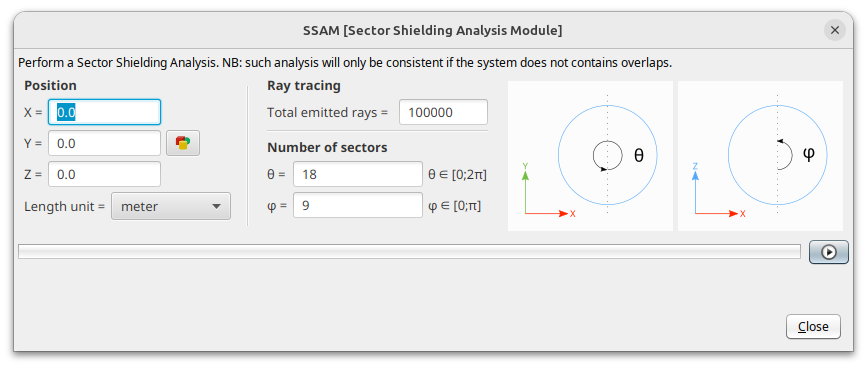
Position: It is necessary to select a position where to perform the sector shielding analysis. It is represented as \$x\$, \$y\$, \$z\$ and a length unit for the position. The button enables to define position easily, see Position parameters.
Sphere sectors: It is needed to provide a number of sphere sectors to divide the space in theta(\$θ\$) and phi(\$φ\$) directions — with theta varying between \$0\$ and \$2π\$ and phi between \$0\$ and \$π\$.
Emitted rays: The total number of rays to launch for the sector shielding analysis.

From the defined position, the selected number of rays is launched in all directions (using an isotropic distribution). SSAM computes the distance in each material density type crossed by the ray and calculates the equivalent thickness of Aluminium defined by a density of \$2.699 g/cm^3\$.

All these results are then summarised for each sphere sector computing the minimal, mean and maximal of the equivalent thickness of Aluminium.

Position parameters

There are several solutions to select position where the computation will happen. The following details how to set up one positions, more details on handling of several positions and parametric positions are provided in SSAM Multi-position dose section.

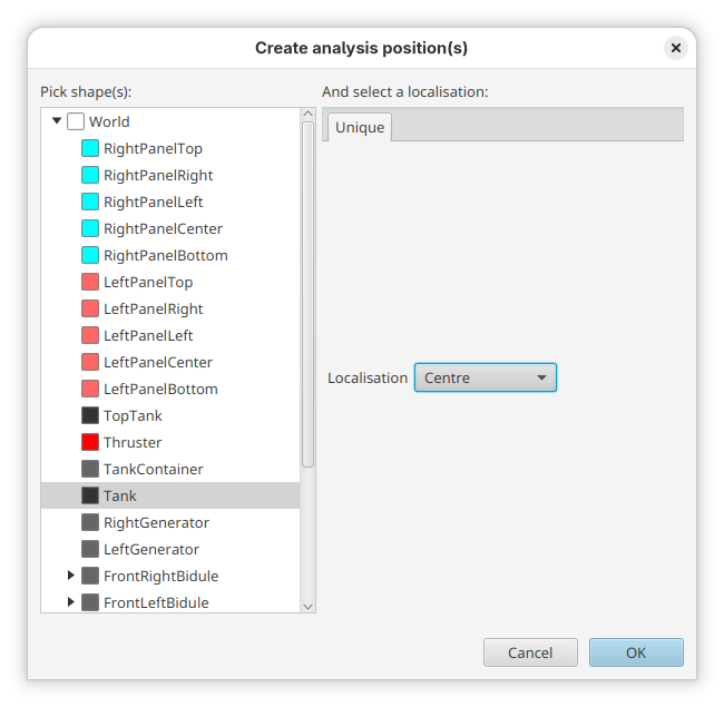
Figure 1. Create single position dialogue

The above dialogue is shown to help define input position for SSAM analysis. It enables to select a shape from the CAD definition (a real shape, assemblies cannot be used in this case). Once a shape is selected, it is possible to select simple position within the shape, the following options are possible:

at the shape centre (so its defined position)
on its surface at \$-X\$, \$+X\$, \$-Y\$, \$+Y\$, \$-Z\$ or \$+Z\$.

When btn:[OK] is clicked the selection is converted to the X/Y/Z position to be used.

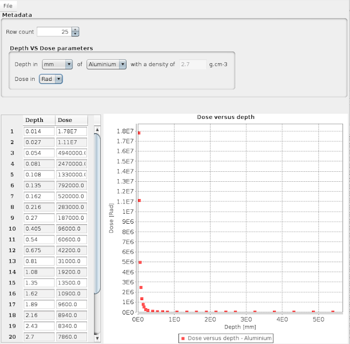
Dose parameters

As noted before, to perform a dose computation, users must beforehand compute the tabulated function defining the evolution of the cumulative dose versus the depth of a material, using external software, models or experimental data for the wanted environment. The user may, for instance, use the Shildose2 model, as provided in the frame of the ESA/BIRA/Spenvis online application.

Then it is possible to set the needed parameters for dose computation:

Dose versus depth curve: It is possible to set it manually directly in the editor or to load a CSV file with two columns separated by a comma (to do so, go to menu:File[Load]). The first column defines the depth and the second one the dose. An example of such file is provided in the CSV file for dose example annex and also in the data directory of EDGE.
Depth unit: The depth value (first column) unit must be set between \$g/cm²\$ or millimetre of a material with a specific density for the depth. If the selected unit is \$g/cm²\$, then it is not necessary to set the density because the results do not depend on the density of the material.
Dose unit: The dose value (second column) must be set between \$Gray\$ or \$Rad\$.

As shown below, the selected parameters are dynamically interpreted to display on the right part of the editor the points of the tabulated function.

Figure 2. Dose parameters view

SSAM Single mode

In single mode, at startup it is needed to provide one position, the number of sectors and rays as presented in previous section. Then click on btn:[Play] button to launch SSAM.

Figure 3. Inputs parameters for SSAM in single mode

SSAM results are displayed after all the rays are launched.

There are several areas to display SSAM results as illustrated below.

Figure 4. SSAM results

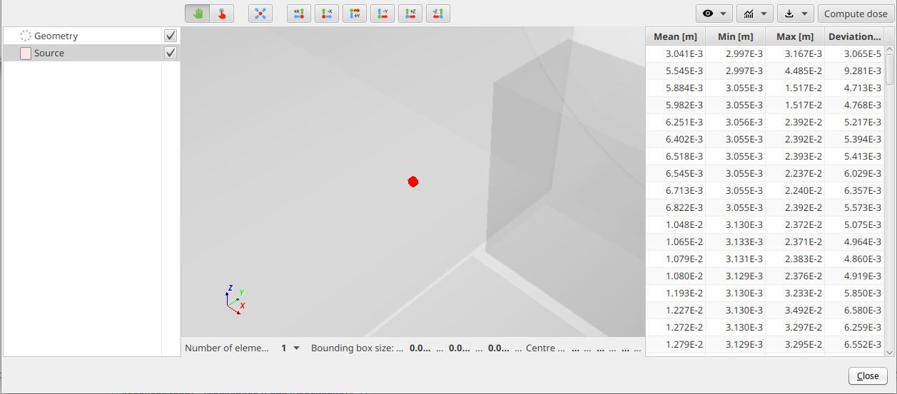
Left: Lists the 3D results elements and allow to change their visibility, transparency and colours by clicking on the corresponding checkboxes and coloured buttons. By default, the modelling geometry is displayed in transparency and in black colour. The position of the target is represented by a red sphere. Please note, in some cases, this sphere can be small compared to the global geometry size and a zooming might be needed to see it.
Centre: 3D view of the different results computed with SSAM.
Right: Table with 4 columns and several rows. Each row is the result of a sphere sector defined by a division in theta and phi directions described by the input parameters. The columns are respectively the mean, the minimum, the maximum and the standard deviation of the mean values of the equivalent thickness of aluminium in this sphere sector. All these values are expressed in metre.

The standard deviation is computed with the formula below, where $nb_{rays}$ is number of rays launched in the sphere sector, $t_{i}$ is the equivalent thickness of the ray $i$ and $t_{mean}$ the mean of all equivalent thicknesses in the sphere sectors:

\$deviation=\sqrt{\frac{\sum_{i=1}^{nb_{rays}} (t_i - t_{mean})^2}{nb_{rays} - 1}}\$

Top right: The contextual menu bar provides several possibilities to display the selected results in the 3D view or as plots, export them into CSV format files or to compute the dose received by the target. More details on these actions are available in the next section.

3D results

The Show 3D button button menu allow to display results in the 3D view. The selected result appears in the 3D view and is listed in the control panel.

The following 3D representations are available:

The minimum, mean or maximum of the equivalent aluminium thickness for each sphere sector. More information about each sphere sector can be obtained by clicking on each sphere sector item in the list of 3D items;

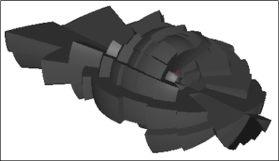Figure 5. 3D sphere sectors results or "hedgehog view"
The average sphere considering the mean of the equivalent aluminium thickness for all rays launched by SSAM. The details regarding this sphere, like the diameter can be displayed by clicking on the item in the list of 3D items.

The information bar at the bottom of the 3D view gives the size of the selected element bounding box enabling to quickly access the size of the sphere;
The number of interceptions for each face of the geometry. This 3D result can be used to check if enough rays have been launched to provide a statistic good enough: if a face has zero interceptions, it indicates that not enough rays has been launched to intercept this face.

When selecting this results in the list of 3D items, a scalar bar appears helping assess the value represented by each colour;

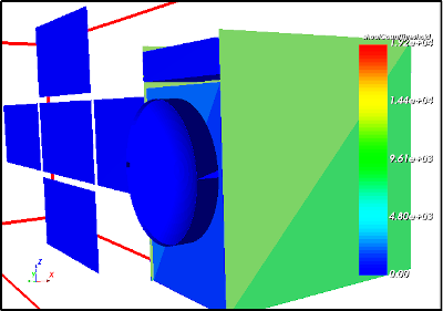Figure 6. Number of intercepting rays for each face
The minimum, mean or maximum hollow sphere sectors of equivalent aluminium thickness. Users must set the inner radius of the hollow sphere, and the space between each sphere sector. The details of each hollow sphere sector are available by clicking on each sphere sector item in the list of 3D results.

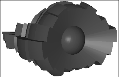Figure 7. 3D hollow sphere sectors results
A coloured sphere where each colour represents the value of the equivalent thickness of Aluminium in metre.

When selecting this results in the list of 3D items, a scalar bar appears helping assess the value represented by each colour.

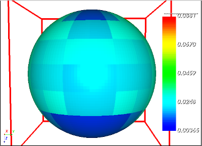Figure 8. Sphere sector aluminium equivalent thickness mapped on a coloured sphere

Plot results

The Show plot button button menu enables to display plots of meaningful results into a pop-up window.

The following results are available:

$y = f(x)$ chart type where the minimum, the mean and the maximum of the equivalent thickness of Aluminium in metre for each sphere sector is displayed.

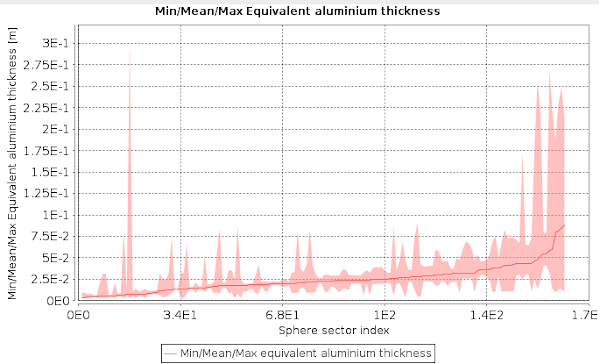Figure 9. Minimum, mean and maximum equivalent thickness of Aluminium in metre for each sphere sector
$y = f(x)$ chart type with the mean of the equivalent thickness of Aluminium in metre and its standard deviation are displayed for each sphere sector.

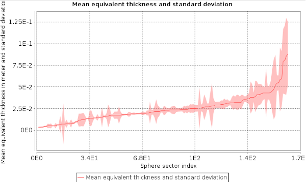Figure 10. The mean of the equivalent thickness of Aluminium and its standard deviation in metre for each sphere sector
A 2D Map showing the angular repartition of the equivalent thickness of Aluminium for each sphere sector.

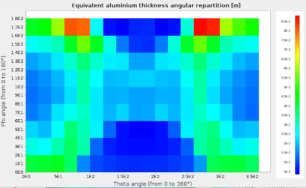Figure 11. Angular repartition of the equivalent thickness of aluminium in metre for each sphere sector

Export options

The Export button button menu enables to save the following results on the disk:

The equivalent thicknesses of Aluminium in metre to a CSV file;
An equivalent sphere with a radius equal to the average of the equivalent thicknesses of Aluminium of all rays used for SSAM.

This sphere is exported to a GDML file;
The number of rays which intercepted each face of the geometry in a VTK file;
The hollow sphere sectors using the minimum, the mean or the maximum of the equivalent thickness of Aluminium of all sphere sectors.

The hollow sphere sectors are exported to a GDML file.

Users must set the radius of the hollow sphere, and the space between each sphere sector to avoid cross contacts and overlapping between sectors to respect GEANT4 constraints.

Dose computation

The Compute dose button enables to compute the cumulative dose based on the previous computed aluminium equivalent thicknesses.

When clicking on it, the Dose parameters window appear.When the inputs parameters for the dose computation are set, users can click on the Compute dose button to launch the computation.

Then a new popup appears with the results of the cumulative dose.The results are computed considering the minimum, the mean and the maximum of the equivalent thickness of Aluminium for all sphere sectors.

Users can choose to save these results in a dedicated file by clicking on the Save button.

SSAM Multi-position dose

In multi-position mode, at startup it is needed to provide the positions, the number of sectors and rays as presented in previous section and the dose-depth data.

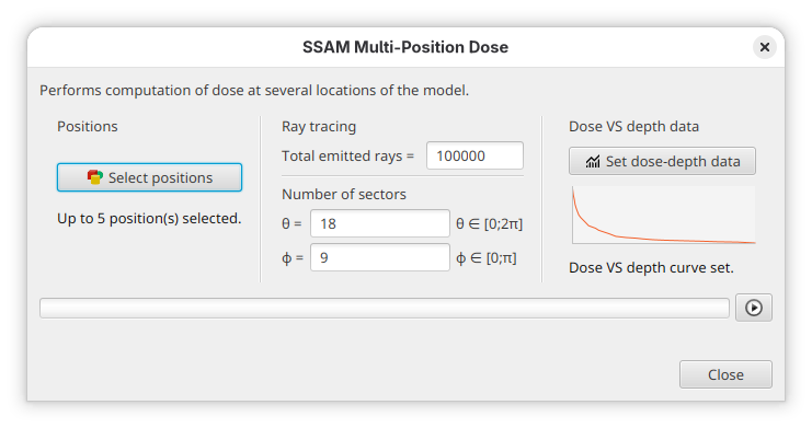
Figure 12. Inputs parameters for SSAM in multi-position mode

To set the positions, click on the btn:[Select positions] button. It will open the multi-position selection dialogue where the positions can be selected.

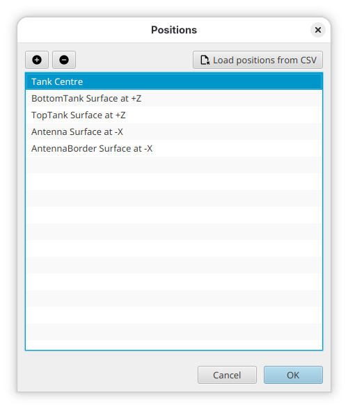
Figure 13. Positions selection dialogue

In this dialogue, positions can be easily added with Add position button or removed with Remove position button .

When adding a new position, a new dialogue appears to select a position as presented in Position parameters. An additional tab is present to add parametric positions as presented below.

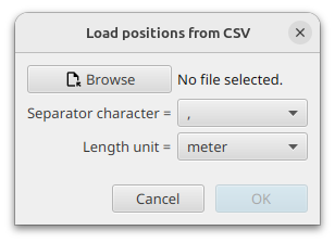
Additionally, the btn:[Load positions from CSV] button enables to load the positions from a given CSV file. This file must have with three columns for \$x\$, \$y\$, \$z\$. When clicking the button, a small pop-up as shown below appear to select the file, the element separator inside the CSV file as well as the position unit.

Figure 14. Load from CSV pop-up

Parametric positions

When computing several positions with multi-dose, an additional tab is available to select parameteric positions.

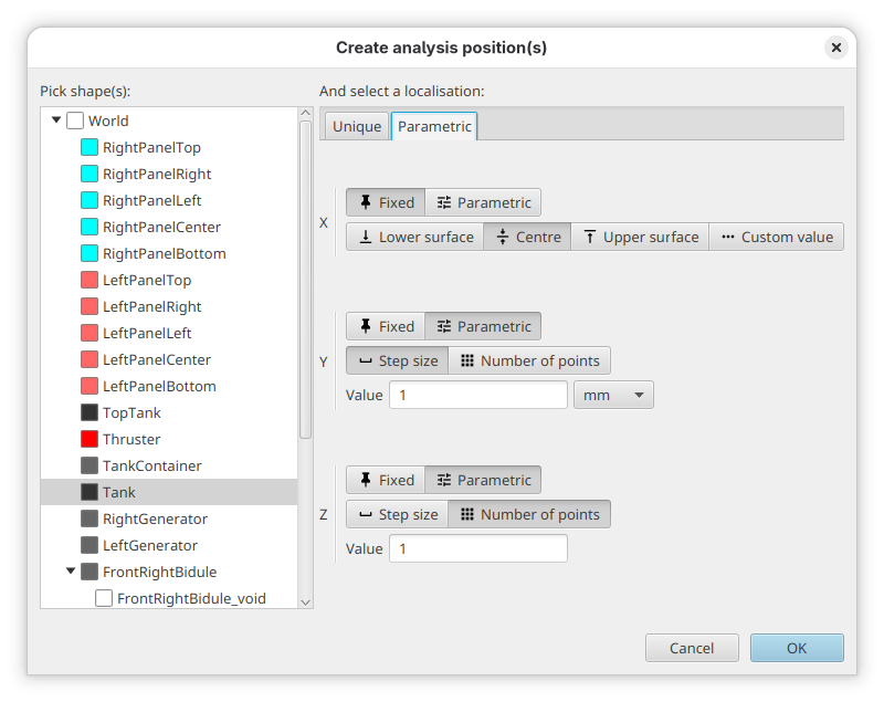
Figure 15. Create a parametric position panel

Once a shape is selected, there are several options to create positions from a shape with parametric options.

To improve automatic results, it is recommended to use parameteric options for two axes maximum and fixed on one axis at least.

When the Fixed position button button is selected, for each axis the available options are similar that one position ("lower" surface, centre and "upper" surface). An additional option enables to provide a custom location along the axis.

When the Parametric position button is selected, two options are possible:

Step size: The provided value indicates the step between two successive points on the current axis. A chooser enables to select the unit of the step value.
Number of points: The provided value is the total number of points that will be created along the axis.

Taking into account all the provided values and the shape, the final positions will be created. For parametric values, the first position will be located at \$step/2\$ from the minimum size of the shape on the given axis. All possible points using the provided parameters will be created.

Run multi-dose and results panel

Then click on btn:[Play] button to launch SSAM for each selected position. If numerous positions are set up, the computation can take some time to finalise.

All dose results are displayed after all the rays are launched for each position.

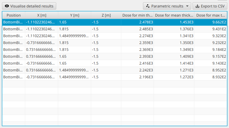
Figure 16. Results panel for SSAM in multi-position mode

The first column provides a name for the position indicating how it was computed, the next three columns display the selected position \$x\$, \$y\$ and \$z\$ components in metre. The last three columns present the dose results with the minimum, mean and maximum dose for the selected position.

By selecting a specific line of the table, it is possible to see detailed results with btn:[Visualise detailed results]. It will display the same interface as the single mode result.

If a parametric position was set up, it is possible to visualise summary results by clicking on btn:[Parametric results], select the wanted parametric result and whether results should be displayed for min/mean/max thickness of material. If one axis was set up as parametric, the result will be a XY plot, otherwise, for two axis, the result will be displayed as a 2D colour map. It is not possible to display such results if all axis are parametrised.

As for single position, it is possible to export the results to a CSV file by clicking on the btn:[Export to CSV].